EU carbon prices signal high policy credibility and farsighted actors

The model LIMES-EU

All quantitative results in this work are obtained using the model LIMES-EU (Long-term Investment Model for the Electricity Sector), version 2.38. LIMES-EU is a linear optimization modelling framework that simultaneously determines cost-minimizing investment and dispatch decisions for generation, storage and transmission technologies in the European electricity sector. Although its clear focus is the electricity sector, the energy-intensive industry and district heating are also represented through marginal abatement cost curves. Compared with simple emissions trading models with static exogenous cost abatement curves, using an energy system model such as LIMES-EU allows to assess not only market developments (for example, prices or allowances in circulation) but also the investment dynamics and path dependencies within the electricity sector.

LIMES-EU allows to fully simulate the EU ETS including the Market Stability Reserve (MSR)⁵¹. Hence, one can analyse figures such as the number of allowances in circulation, the intake by the MSR and resulting carbon prices. By varying the cap and MSR parameters, one can reproduce the state of the EU ETS between different political reforms.

A comprehensive description of the LIMES-EU model, including parameters, equations and assumptions, is provided in the documentation available from the model’s website⁵².

All changes to LIMES version 2.38 made for the purposes of this study are described below.

A myopic version of LIMES-EU

Rolling horizon as operationalization of myopia

Originally, LIMES-EU was formulated as a perfect foresight model running in five-year steps from 2010 until 2070. For the purpose of this study, to simulate the effect of myopic behaviour of decisionmakers, we extend the model with the option to use rolling time horizons instead of full intertemporal foresight. Mathematically this means that instead of solving one optimization problem over the whole time period from 2010 until 2070, we solve multiple (consecutive) optimization problems, covering shorter time periods.

In our choice to implement a rolling horizon, we follow several other publications from our field: the rolling horizon approach (that is, short foresight with overlapping time steps) has already been used extensively as a way to represent myopia in the context of energy systems modelling^41,43,44,47. Although principally other approaches would be possible (for example, by varying the discount rate), we are not aware of any publication in our field representing myopia in a different manner.

Foresight length

All myopic foresight results in this work assume ten-year horizons with an overlap of five years between the horizons. Practically it means, actors have foresight of ten years but can revise their decisions every five years. As LIMES-EU runs in five-year time steps, one optimization horizon comprises always two time steps (for example, (2020, 2025), covering years 2018–2027).

The literature provides different estimations on planning horizons of manufacturing companies, ranging between three and 12 years⁶. Bocklet and Hintermayer⁶ and Quemin and Trotignon⁷ show that a horizon of around ten years can best replicate EU ETS developments (these analyses were conducted around the time of the MSR reform). Hence, we also chose a foresight horizon of ten years. As our model runs in five-year time steps, ten years is also the shortest foresight horizon we can meaningfully implement (that is, which allows for an overlap) in LIMES-EU. Varying the length of the foresight horizon impacts the results but not the general trends: the shorter the foresight, the lower the near-term carbon prices and higher the delays in decarbonization⁴⁷.

When running in myopic foresight, the model solves consecutively several individual optimization problems. Still, some variable values computed in one optimization horizon need to be transferred into the next optimization horizon. It concerns all previous capacity additions and decommissioning (needed to correctly compute current capacities) and emissions and banked certificates (needed for the ETS/MSR simulation). For instance, for the optimization horizon (2020, 2025) capacities will be fixed for 2020 and all time steps before 2020. We assume that dispatch decisions can still get revised every time step (five years), so for example, for the optimization horizon (2020, 2025), emissions and banked certificates values get fixed only for all time steps before 2020 but not 2020 itself.

What do actors neglect and what do they still consider

In our study, we use rolling horizons as a tool to represent actors’ myopia due to low trust in the long-term stability of the EU ETS. Hence, our main aim is to depict actors that are myopic with regards to the ETS. Our modelling approach implies that actors don’t consider any information outside of their ten years foresight horizon (that is, the future ETS cap and the future demand for certificates).

Nonetheless, as ETS actors are mostly large power system or manufacturing companies and salvage values (‘book values’) are traditionally part of companies balance sheets, we still assume that they consider the future value of capacities also beyond the foresight horizon. Therefore, a salvage value for the capacity stock remaining at the end the optimization horizon is subtracted from the cost function. In the myopic version, the salvage value is considered in each time horizon. This means that when we run a diagnostic scenario where we turn off the ETS and keep technology prices constant over time, the results of the myopic mode exactly reproduce the results of the perfect foresight mode.

MSR simulation

The MSR, which is originally implemented iteratively as a loop around the main optimization problem⁵¹, runs in the myopic model version around each time horizon.

Specific modelling aspects

Carbon prices

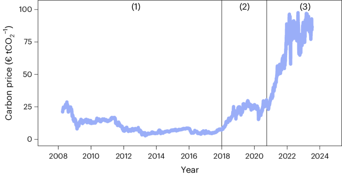
Reported carbon prices (in € tCO₂⁻¹) represent the marginal abatement costs in a given year, which are equal to the dual value (shadow price) associated with the banking constraint in LIMES-EU. Transaction costs are neglected. Reported historic carbon prices are nominal, so given in € of the year in which they occurred. LIMES runs in real €₂₀₁₀, but all reported prices from LIMES until 2023 in this paper were converted to nominal prices until 2023, adjusted for inflation using inflation rates provided by the Organization for Economic Co-operation and Development⁵³. Computed prices after 2023 are in real €₂₀₂₃.

External investors

To depict external investors in our model, we assume that the impact on carbon prices of buying/holding/selling EUA futures can be approximated by the assumption, external investors buy/hold/sell physical allowances. As we are interested in long-term price developments, we focus on external investors holding long open position on EUA futures.

To model the impact of external investors, we implement a one-step iteration approach. Hence, we implicitly assume that both compliance actors and external investors can’t react the other group’s action.

(1) In a first instance, a LIMES-EU run with full myopic foresight without external investors is conducted.

(2) The resulting carbon price trajectory \({p}_{{{\mathrm{price}},{\mathrm{CO}}}_{2}}({t}_{\mathrm{{y}}})\) serves as input to the optimization problem from the external investors’ perspective:

Equation (1) is the profit function: external investors want to maximize their profit by buying allowances and selling them at a later time step \({t}_{\rm{y}}\). Herein, \({t}_{\mathrm{y}}\in [2018,\ldots ,2040]\) are yearly time steps. T is the set containing all yearly steps part of the optimization. Further, \({v}_{\mathrm{bought}}({t}_{\mathrm{y}})\) and \({v}_{\mathrm{sold}}({t}_{\mathrm{y}})\) stand for the number of allowances bought and sold in time step \({t}_{\mathrm{y}}\). The profit gets discounted by discount rate i. We assume i = 5%, same as in the core model assumptions of LIMES-EU. Finally, \({p}_{{{\mathrm{price}},{\mathrm{CO}}}_{2}}\left({t}_{\mathrm{y}}\right)\) corresponds to the carbon price from a myopic run, which grows at a higher rate than the discount rate of 5%.

Equation (2) sets a limit on the number of allowances external investors can maximally buy. Herein, \(\alpha\) is the share of auctioned allowances \({p}_{\mathrm{auction}}({t}_\mathrm{y})\). We assume \({p}_{\mathrm{auction}}\) to be the final number of allowances auctioned, after subtraction of allowances transferred into the MSR. In our work, \(\alpha\) is varied between 5 and 20%. Equation (3) ensures the number of allowances sold is below the number of allowances external investors bought prior to time step \({t}_\mathrm{y}\).

Finally, equation (4) limits the number of allowances that can be sold in a given time step \({t}_\mathrm{y}\), to prevent all of them being sold in a single year. Results assume an \(\gamma\) of 0.2, meaning allowances need to be sold over minimum five years.

(3) Having solved the optimization problem from the perspective of external investors, one can now conduct a new LIMES-EU run with full myopic foresight and additional input on the number of allowances blocked by external investors.

Here \({p}_{\mathrm{investors}}\) is the absolute number of allowances bought or sold by external investors. These influence the level of allowances, as shown in equation (7). Here \({v}_{\mathrm{tnac}}(t)\) is the total number of allowances in circulation (TNAC) at the end of time step t, \({p}_{\mathrm{cap}}(t)\) the total number of allowances auctioned and freely allocated and \({v}_{\mathrm{emi}}(t)\) the total emissions in time step t. Here \(t\in [2010,2015,\ldots ,2040]\) are five-year time steps.

To capture the unpredictability of external investors on the price formation, we assume compliance actors can’t see the realization of \({p}_{\mathrm{investors}}\left(t\right)\) before time step t. Hence, even though they have a foresight of ten years regarding all other model inputs, they only have a foresight of one LIMES-EU time step (five years) when it comes to \({p}_{\mathrm{investors}}\left(t\right)\).

It is important to note that the way our approach is implemented, external investors behave as farsighted actors and have incentives to enter the market, only if compliance actors are myopic (carbon prices initially lower than under the perfect foresight scenario). Hence, all results showing the impact of external investors presume myopic foresight from compliance actors.

As we conduct only one iteration, we implicitly assume that external investors plan all their future behaviour only once and base it on myopic carbon prices. In the real world, there is a constant feedback between prices and investors’ buying/selling strategy. Hence, our methodology does not aim to provide realistic predictions regarding possible behaviour of external investors. It is, however, suitable to show the order of magnitude of the increase in carbon prices, assuming external investors block a certain number of certificates.

Future

In the ‘Reversal to myopia’ scenario from Fig. 5b, similar to the full myopic version, several consecutive optimization problems with ten years foresight horizons are solved, with the exception that the horizon [2020, 2025] gets replaced by [2020,…, 2070] to simulate perfect foresight in time step 2020. Afterwards, from time step 2025 on, actors have again only myopic foresight.

MACC curves representing industry and heating sectors

As described in the LIMES-EU Documentation⁵², the industry and heating sectors are not modelled explicitly in LIMES-EU, but the cost of emissions abatement is approximated by marginal abatement cost curves (MACCs). Originally, as they have been designed for runs starting in 2020, both MACCs assumed a minimum cost of €8 tCO₂⁻¹, being a well-suited assumption for benchmark modelling, in which modelled carbon prices always exceed €8 tCO₂⁻¹ for relevant ETS scenarios. As in this work certain counterfactual scenarios yield prices below €8 tCO₂⁻¹_, we extrapolate the MACC curves to also cover the price regime of €0–8 tCO₂⁻¹ by analysing the change in industry and heating emissions upon implementation of the ETS. We thus estimate two additional emissions steps of 45 Mt CO₂ in industry and 15 Mt CO₂ in heating that would be emitted additionally compared to historic industry/heating emissions when ETS prices remain below €5 tCO₂⁻¹ and again when they remain below €3 tCO₂⁻¹.

Scenarios

Modelling assumptions regarding calibration, policy targets and technology costs

The key assumptions behind our study’s main scenario types are summarized in Extended Data Table 3. In Fig. 3, we align scenarios with historical conditions as closely as possible, adjusting variables such as ETS modelling start year and technology cost assumptions. Due to the five-year time steps in our model, complete historical replication and path dependency coverage may be limited (for example, ‘Fit for 55’ scenario starts in 2018).

For Figs. 4, 6 and 7, we exclusively use the ‘Fit for 55’ scenario, representing the current EU ETS state. This simplification serves the purpose of preventing information overload, aligning with the figures’ primary objective. In Fig. 6, we extrapolate our results to 2015.

‘Fit for 55’ Commission’s proposal vs final agreement

Extended Data Table 4 summarizes the relevant parameters used in this study defining the emissions cap and MSR functionality for the ETS state between different reforms.

All results in this study related to ETS targets from the ‘Fit for 55’ package assume parameters from the Commission’s proposal published in July 2021⁵⁴. As this study takes into account real ETS prices until December 2022, it is plausible to assume that until then market actors were basing their decisions on the Commission’s proposal, not being aware yet of the upcoming changes in the final negotiations.

For completeness reasons, we provide a comparison of modelled carbon prices according to the emissions cap from the Commission’s proposal (used in this study) and according to the emissions cap from the final ETS ‘Fit for 55’ agreement^39,55 in Extended Data Fig. 4. The emissions cap corresponding to the final agreement can be found in Extended Data Table 2.

Model validation

General modelling choices, for example, the clustering approach and the representative days choice, are described in the LIMES-EU model documentation. Here we present additional validation points for the scenarios presented in this study. First, we show that our model can approximate historical developments in 2015 and 2020. Then, we provide references demonstrating that our future estimates for the EU ETS align with other literature.

Reproducing historical developments in time step 2015

The capacity spin up of LIMES-EU is fixed so that it matches the 2015 historical mix of installed generation capacities in EU ETS countries. Extended Data Fig. 5 illustrates that based on this standing capacity, the model-calculated dispatch then reasonable matches the historic power generation dispatch in EU ETS countries. The total modelled emissions from electricity generation in the year 2015 for EU ETS countries covered by LIMES-EU amount to 981 Mt CO₂, closely aligning with the historical emissions of 967 Mt CO₂ reported by Mantsos et al.⁵⁶ Because emissions from industry, heating and aviation are also calibrated to match their historical 2015 levels (as described in LIMES-EU documentation⁵²), this calibration ensures that our model generates meaningful values for total emissions in the 2015 time step. Also, the model-endogenous investments in 2015 lead to standing capacities in 2020 that match historic wind and solar capacities in 2020. To this aim, we additionally assume subsidies for electricity generated from solar or wind sources (€0.04 kWh⁻¹ for solar and €0.015 kWh⁻¹ for wind) to represent the various renewable subsidies that were in place in most EU member states. Our model, however, underestimates the capacity additions of offshore wind until 2020, which took place mostly in the United Kingdom.

Reproducing historical developments in time step 2020

To validate the 2020 model results, we first fix capacity spin up so that our model matches the installed generation capacities for both 2015 and 2020 in EU ETS countries. In Extended Data Fig. 6, we show that this calibration enables our model to approximate EU-wide dispatch and total emissions from the electricity sector in 2020. It’s important to note that our model operates in five-year steps, with time step 2020 representing the actual years 2018–2022. However, due to the exceptional circumstances of the COVID-19 pandemic, the year 2020 deviates from the typical trends of 2018–2022. Hence, to validate time step 2020, we provide real values for the years 2019 and 2020.

With respect to electricity dispatch, our model estimates lower generation from biomass compared with the International Energy Agency (IEA) historical data. This discrepancy may be attributed to several factors, including our reliance on the European Network of Transmission System Operators for Electricity (ENTSO-E) dataset for total capacities, whereas using the IEA dataset for generation values (as ENTSO-E lacks a Statistical Factsheet covering generation for the years 2019 and 2020). Differences in values from different sources can often be substantial. Regarding biomass, variations may be due to, for example, the way biomass co-firing in coal power plants is accounted for. Nevertheless, despite minor deviations in our 2020 electricity dispatch from historical data, our model still provides a meaningful estimate of emissions. This aspect is critical for validating EU ETS models, as it directly impacts CO₂ prices, the total number of allowances in circulation and the functioning of the MSR.

Estimating future developments

While validating future projections is inherently impossible, we observe that LIMES-EU generally aligns with findings in the literature and does not produce results that are far outliers compared with other models. Osorio et al. discuss that LIMES-EU’s estimates of MSR cancellations are consistent with other studies⁵¹. Furthermore, a recent model comparison study led by Henke et al. revealed that LIMES-EU’s projections for various EU electricity sector variables from 2020 to 2050, such as final energy demand and the share of renewable energy sources in electricity generation, are in line with the range provided by ten other energy systems and integrated assessment models⁵⁷. In another model comparison study assessing EUA prices until 2030, LIMES-EU’s estimate of €140 tCO₂⁻¹ falls within the range of €80 to €160 tCO₂⁻¹ produced by six different models⁵⁸.

Methodological contribution

Whereas the primary focus of this work lies in providing insights for the ongoing debates surrounding the EU ETS, we also make a notable methodological contribution. There have been other studies using EU ETS models that explicitly simulate the electricity sector^33,59,60, and there have been energy systems analyses using myopic energy system models^41,43,44,47. Also Nerini et al.⁴⁷ pioneered the idea to compare myopic and perfect foresight modes of a capacity expansion model to formulate more robust policies. Our study extends their approach and employs both types of foresight to evaluate ex post a concrete policy reform to test whether the change in the observable variable—in our case, the EU ETS price—can better be reproduced in the myopic or perfect foresight mode.